Sunday, February 21, 2010

DSP Tutorial #11: Loading, Plotting WCDMA Signal


The raw WCDMA signal can be located on the menu to the right, or by using the link below:

DSP: WCDMA File (wcdma2.csv)

The sample frequency used to sample this signal was fs=32496000

The following code loads the signal and produces a time series plot.


%% Loading WCDMA 3G Signal
close all;
clear all;
fs=32496000; %sample frequency
x=load('wcdma2.csv');
figure('Color',[1 1 1]);
plot(x);
axis('tight');
title('Time Domain Plot of WDMA Modulated Signal');

DSP: Tutorial Post #10: Windowing


- DFT can only be performed over a finite-time sample interval

- We can think of the DFT input singal as the product of an input signal existing for all time and a rectangualr window whose magnitude is 1 over the sample interval

- Anytime we take the DFT of a finite-extent input sequence we are, by default, multiplying that sequence by a window of all ones and effectively multiplying the input values outside the window by zeros

- Remember: The continuous Fourier transform of the rectangular window IS the sinc function

Windowing premultiplies input data supplied to the FFT with a value that smoothly decreases to zero at each end of data. The purpose is to reduce "leakage" aberrations in the FFT output that are introduced by sudden changes in the data at the start and end of data. Windowing reduces DFT leakage by minimizing the magnitude of the sinc function’s sin(x) / x sidelobes. This is accomplished by forcing the amplitude of the input time sequence at both the beginning and the end of the sample interval to go smoothly toward a single common amplitude value. (taken from Understanding Digital Signal Processing – Lyons).

Matlab supports the following windows:
barthannwin,bartlett, blackman,blackmanharris,bohmanwin,chebwin,flattopwin,gausswin, hamming,hann,kaiser, nuttallwin,parzenwin,rectwin,triang,tukeywin

In this example we will compare the sidelobes created by the rectangle window as compared to the blackman window.


%% Example of Windowing
close all;
clear all;
% Example of windowing
freq = 12; % continues time signal frequency in Hz
fs=800; % sample frequency 800Hz (how many samples per second)
Ts=1/fs; % sample period (time between consecutive digital captures of the continues time sigal)
n=0:1*fs; % sample index (fs=samples per second), 2 second (how long to watch the signal)
tn=n*Ts; % our x axis, descrete measurements
x=cos(2*pi*freq*tn); % create signal
w=blackman(length(x)) % create a blackman window the same length as x(t)
c = x.*w'; % multiply our signal and window, the ".*" completes element by
% element multiplication. The "'" transposes our window matrix
figure('Color',[1 1 1]);
plot(tn,c,tn,w,'--r');
title('x(t) windowed with Blackman');
axis([-.5 1.5 -1.5 2.5]);
% Freq domain plot
[Y,f]=ComputeSpectrum(x,fs,2^14);
[X,f]=ComputeSpectrum(c,fs,2^14);
figure('Color',[1 1 1]);
plot(f,20*log(Y),f,20*log(X),'--g');box off;hold on;
xlabel('Frequency');
ylabel('Amplitude');
title('Spectrum w/ Window');
axis('tight');
legend('Rectangular Window','Blackman Window');

Sunday, February 14, 2010

DSP Tutorial #6: Looping in Matlab


Looping is helpful if we need to repeat certain specific commands. In this example we will use the for loop to create a sinusoid of various frequencies as a function of the loop variable. The following code creates six (6) plots, each with a different 'frequency' as determined by the conditional if statement based on our loop variable i.

close all;
clear all;
for i=1:6;
if i==1,freq=10;,end;
if i==2,freq=25;,end;
if i==3,freq=50;,end;
if i==4,freq=75;,end;
if i==5,freq=100;,end;
if i==6,freq=125;,end;
fs = 8000;
Ts=1/fs; % sample period
n=0:1*fs; %sample index (fs=samples per second), 1 second
tn=n*Ts;
x=cos(2*pi*freq*tn);
% Time domain plot of x(t)=cos(2*pi*5*tn)
figure('Color',[1 1 1]);
h=plot(tn,x);box off;
xlabel('Time(s)');
ylabel('Amplitude');
title(['x(t)=cos(2*pi*freq*tn) in the time domain (freq=',num2str(freq),'Hz)']);
end;

Friday, February 12, 2010

DSP: Lowpass Elliptical Filtering

The following function creates a lowpass elliptic filter. By implementing this filter in a function we can easily call the lowpass filter in our code, passing our signal "x", sample frequency "fs", and desired cutoff frequency "fc".


function [y,N,B,A]= lowpass(x,fs,fc);
% Description: This function uses an elliptical filter
% to filter out high frequencies.
%
% [y,N,B,A] = lowpass(x,fs,fc)
%
% Variable Definition:
% x: Input signal
% fs: Input signal sampling frequency in Hz
% fc: cutoff frequency
%
% y: Filtered signal (output)
% N: Filter order
% B: Feedforward (FIR) coefficients
% A: Feedback (IIR) coefficients
Rp = 0.5; % Ripple in dB (passband)
Rs = 20; % Attenuation
mf = fs/2; % Maximum frequency
Wp = fc/mf; % Cuttoff frequency
Ws = 1.2 * Wp; %Stopband frequency
% First, determine the minimum filter order to meet specifics
[N,Wn] = ellipord(Ws,Wp,Rp,Rs);
% Next, Design the filter (find the coefficients)
[B,A] = ellip(N,Rp,Rs,Wn,'low');
% Now, apply the filter (filter the signal)
y = filtfilt(B,A,x);
% Plot the filter
figure('Color',[1 1 1]);
freqz(B,A,2^14,fs);

Wednesday, February 10, 2010

DSP: Noise Averaging WCDMA Example

The following example show noise averaging affects for a WCDMA signal. Coherent averages were taken of a WCDMA signal with additive noise k=.1.

The first plot shows a pure WCDMA modulated signal with additive noise.

Next, the signal is plotted with three (3) noise averages:


Finally, ten (10) averages are simulated:


The plot below shows a zoomed in area of the shoulder.

Saturday, February 6, 2010

Audio Processing Using Basic DSP Techniques
Prepared by: James Eastham, Member IEEE

In this tutorial we will use an audio signal as a practical example of common DSP techniques. We will apply the concepts of sampling, time-domain analysis, spectral analysis, and digital filtering. We will load an external sound file in wav format into Matlab for this analysis. Basic Matlab plots will be used to display our results. The Spectrogram will also be introduced.

Before we start, let’s review audio frequencies. Taken from Wikipedia: “An audio frequency is characterized as a periodic vibration whose frequency is audible to the average human. While the range of frequencies that any individual can hear is largely related to environmental factors, the generally accepted standard range of audible frequencies is 20 to 20,000 hertz. Frequencies below 20 Hz can usually be felt rather than heard, assuming the amplitude of the vibration is high enough. Frequencies above 20,000 Hz can sometimes be sensed by young people, but high frequencies are the first to be affected by hearing loss due to age and/or prolonged exposure to very loud noises.

We will use the Wikipedia definition as a guide to help us filter the audio signal.

To load the wav file (Pule Code Modulated file) we use the wavread function in Matlab. We need to know the sample frequency that was used to produce the file to play it at the correct speed. The following code will open the file and play it using the soundsc function.

clear all; %clears all variables
close all; %closes all plots
fs=8000; %sample frequency
Ts=1/fs; %sample period
n=0:3.5*fs-1; %sample index (fs=samples per second), 3.5 seconds
tn=n*Ts;
y = wavread('fp3.wav'); %open the message
y=y(1:28000); % This simply trims the file to the desired length

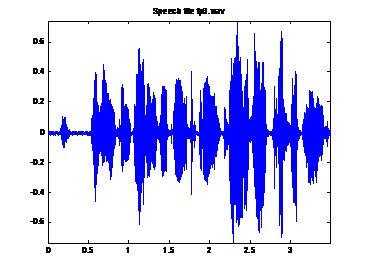
Plotting the Audio File in the Time domain:
The following code will plot the audio file in the time domain.

figure('Color',[1 1 1]);
plot(tn,y);
axis('tight');
title('Speech file fp3.wav');


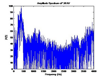
Plotting the Audio File in the Frequency Domain:
The following code will plot the audio file in the frequency domain. This section uses the ComputeSpectrum function we created in a previous blog post. Notice the spectral content, most of the content is below 500Hz. This is good, this is what we expect from an audio signal.


%******** Amplitude Spectrum of *.wav file *************
figure('Color',[1 1 1]);
[X,f] = ComputeSpectrum(y,fs,2^14);
plot(f,20*log(X));
title('Amplitude Spectrum of *.WAV');
xlabel('Frequency (Hz)');
ylabel('|X(f)|');
axis([0 4000 0 100]);

Filtering the Audio File:

Next we will use digital filtering to filter out undesired signals from our audio file. Matlab provides many different filters, in this example we will use the Butterworth filter. To read more about the Butterworth filter see: http://en.wikipedia.org/wiki/Butterworth_filter

The following code implements a tenth order (ten pole) low pass Butterworth filter with a cutoff frequency of 3400Hz. Cutoff frequencies are specified between 0.0 and 1.0 where 1 corresponds to half the sampling frequency: fs / 2 (4000 in our example). For example, for a cutoff frequency of 3400Hz, we specify this as 3400/(fs/2).

fNorm = 3400/(fs/2);
[b,a]=butter(10,fNorm,'low');
filterLow_y=filtfilt(b,a,y);
freqz(b,a,128,fs);
figure('Color',[1 1 1]);
plot(tn,filterLow_y);
axis('tight');
title('Speech file fp3.wav Low Pass Filtered at 200Hz');
soundsc(filterLow_y);
%******** Amplitude Spectrum of filtered *.wav file *************
figure('Color',[1 1 1]);
[X,f] = ComputeSpectrum(filterLow_y,fs,2^14);
plot(f,20*log(X));
title('Amplitude Spectrum of *.WAV');
xlabel('Frequency (Hz)');
ylabel('|X(f)|');
axis([0 4000 0 100]);

The figure below shows the frequency spectrum of the filtered signal; notice how all frequencies above 3400Hz are basically gone now.


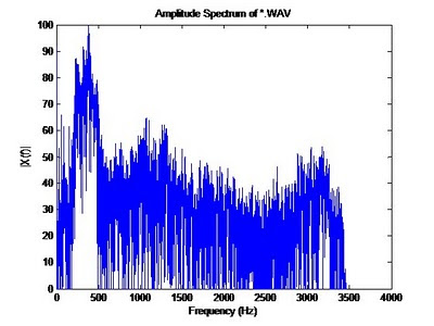
Matlab provides the calculated coefficients if needed for later use or reporting. These are contains in the variables [a,b].

Filtering the Audio File (continued):

Matlab includes function the following Butterworth filters:

* 'low' : Low-pass filters, which remove frequencies greater than some specified value.
* 'high' : High-pass filters, which remove frequencies lower than some specified value.
* 'stop' : Stop-band filters, which remove frequencies in a given range of values.

To implement a ‘high’ pass filter, simply specify the cut off frequency as we did above, and use the ‘high’ keyword in the function call.

To implement the ‘stop’ band, a range must be defined. The following code will define this band. This code basically ‘chops’ out all frequencies from 750Hz to 950Hz.

% bandstop example
fNorm = [750/(fs/2), 950/(fs/2)];
[b, a] = butter(10, fNorm, 'stop');
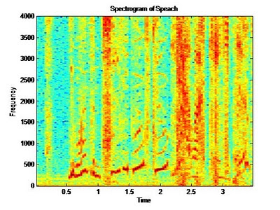
The Spectrogram:

The spectrogram plot allows use to not only see which frequencies are present in our signal, but also when. Basic spectral analysis using the FFT does not allow us to see what spectral content is present at a given time. The spectrogram is a useful tool in spectral analysis. To display the spectrogram, the following code is provided. The 512 below is the number of samples that are used for the DFT, this becomes a grouping factor per column. Think of this as the granularity of the analysis, 512 is typically adequate for analysis. The spectrogram presents interpolated colors of magnitude vs. time. In the plot below, red for example means there is more frequency content at that frequency than say the light blue at a given time. Our audio file contains noise and voice harmonics therefore many frequencies are seen at any given time, however the magnitude of the voice range below 500Hz is see as the darkest (darkest red / black).

figure('Color',[1 1 1]);
specgram(y,512,fs);

Be Careful!!

DSP: Obtaining Raw Stock Data for Analysis


Raw stock data can be obtained by using Google Finance. Search for the stock of interest, and use the "Historical Prices" link on the left. You will see an option to download the data to a spreadsheet. Once you have the spreadsheet downloaded, you can delete the unnecessary columns (only need to keep the close price) and save the file as text for use with Matlab.