Plotting a Discrete Time-Domain Signal in Matlab

In order to properly construct a sinusoid in Matlab we need to do a few things. We need to give Matlab the equation of our sinusoid. We also need to tell Matlab how often to sample the sinusoid and for how long we want to sample our sinusoid. Essentially, we want to tell Matlab “ok, watch this 5Hz sinusoid for 1 second. In that one second, take 50 discrete samples (actually 51), and plot the data. I should see a point every 0.02 seconds, for a total of 51 total points (Matlab starts at zero).” What we want to do may seem pretty simple but this process often confuses students. This overview will help in understanding the proper construction of sinusoids. I say “proper” because we will use the proper DSP terms when we tell Matlab what to do. For example, we will use terms like “sample frequency” and “sample period” to describe our signal.

To establish our signal we will need to:

1. Set the sample frequency FS
2. Set the sample period Ts
3. Set the time window (number of samples)
4. Set the sample index Tn (time index)
5. Establish the signal x(t) and plot
   
   

1. Set the Sample Frequency (Fs):

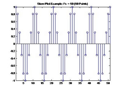
This is our sample frequency. This is basically how many “points” we will use to construct each signal. Remember it’s zero based, so it’s really plus one. In the example below, Fs was set to 50, so we have 51 points in our plot, we ‘sample’ the signal 51 times. This is a 5Hz signal, so we are sampling it 10 times per cycle, which satisfies Nyquist-Shannon’s sampling theorem.

Matlab code:

Fs = 50;

2. Set the Sample Period (Ts):

Next, we will set the sample period, Ts. The sample period is calculated as 1/Fs, or 1/50 in this example = 0.02. This is essentially the ‘granularity’ of our sampling. In other words we will have a discrete point every 0.02 units (which will be time). If we zoom into our signal and only look at the first 0.2 seconds, we can see that we have 11 datapoints, one data point every 0.02s (remember it’s zero based).

Matlab code:
Ts = 1/Fs;

3. Set the Time Window (n):

Next we will establish out how many points are in one second of our signal. We will setup a matrix from zero to one second. In our example Fs = 50, so n = 0:1*Fs. When we set n in Matlab, all we are really doing is setting up a matrix of numbers from 0 to 50. That is: 0,1,2,3,4,5,6,…..,50. We will use this matrix to set the sample index Tn in the next step.

n is now equal to the matrix below:

0 1 2 3 4 5 6 7 8 9 10 11 12 13 14 15 16 17 18 19 20 21 22 23 24 25 26 27 28 29 30 31 32 33 34 35 36 37 38 39 40 41 42 43 44 45 46 47 48 49 50

Matlab code:
n =0:1*Fs;

4. Establish the Sample Index (Tn):

Now we will tell Matlab how to chop up or signal. We set the Sample Index as Tn = Ts * n. In our example, Tn will equal .02. We want to see a discrete point every 0.02 seconds. We will take n, or matrix from 0 to 500 and multiply it by Ts which was 0.02. Now we have a matrix with 51 elements from 0 to 1 spaced every 0.02 seconds. We are now ready to plot our sinusoid.

Tn is now equal to the matrix below:

0 0.0200 0.0400 0.0600 0.0800 0.1000 0.1200 0.1400 0.1600 0.1800 0.2000 0.2200 0.2400 0.2600 0.2800 0.3000 0.3200 0.3400 0.3600 0.3800 0.4000 0.4200 0.4400 0.4600 0.4800 0.5000 0.5200 0.5400 0.5600 0.5800 0.6000 0.6200 0.6400 0.6600 0.6800 0.7000 0.7200 0.7400 0.7600 0.7800 0.8000 0.8200 0.8400 0.8600 0.8800 0.9000 0.9200 0.9400 0.9600 0.9800 1.0000

Matlab code:

Tn =Ts*n;

5. Plot our 5Hz Sinusoid:

Plotting our sinusoid is pretty easy at this point. Remember, we want a 5Hz cosine signal constructed of 51 points in one second; we want to “watch” the signal for 1 second and plot the results. We can plot the X axis correctly with time also using tn.

clear all; %clear all variables

fs = 50; % sample freq

Ts=1/fs; % sample period

n=0:1*fs; % time window (fs=samples per second), 1 second

tn=n*Ts; % sample index

sig_a=cos(2*pi*5*tn);
figure('Color',[1 1 1]);

stem(tn,sig_a);

title('Stem Plot Example: Fs = 50 (50 Points)');

axis('tight');