Tuesday, January 24, 2012

Fourier Transform for Dummies: Matlab Implementation


The following code implements a simple Fourier Transform using cos and sin functions. This project was inspired by a short pdf I stumbled onto during an internet search on this topic. Here is a link to the original: FT for Dummies (I will gladly credit the author if contacted, I just have no idea who wrote the original document as it is not cited)

The following Matlab code, implements a simple Fourier Transform manually in Matlab.

% Fourier Transform for Dummies
% Matlab Implementation
% James Eastham
% Member, IEEE
% 1/22/2012
clear all; %clear all variables
close all; %close all figures
fs = 100; % sample freq
Ts=1/fs; % sample period
n=0:1*fs; % time window (fs=samples per second), 1 second
tn=n*Ts; % sample index
sig_a=5*sin(2*pi*5*tn+pi/3)+2*sin(2*pi*30*tn+pi/2)+2.3*sin(2*pi*8*tn); %create complex signal
sig_a = sig_a + 2*randn(size(tn)); % add noise
figure('Color',[1 1 1]); % plot orignial signal in time domain
subplot(2,1,1);hold on;
plot(tn,sig_a,'-r');
title('Time Domain Signal w/ Noise');
grid on;
% The following loop multiplies the original signal
% by sin and cos at each freq betwen 1 and fs/2
% each sample is then summed, after the loop
% the total sum for each freq is computed
for i=1:fs/2;
detect_sin=sin(2*pi*i*tn);
detect_cos=cos(2*pi*i*tn);
mult_sig_sin=detect_sin.*sig_a;
mult_sig_cos=detect_cos.*sig_a;
total_freq_sin(i)=sum(mult_sig_sin);
total_freq_cos(i)=sum(mult_sig_cos);
end;
total_freq_sin=total_freq_sin/(fs/2);
total_freq_cos=total_freq_cos/(fs/2);
total_freq=sqrt(total_freq_sin.^2+total_freq_cos.^2);
subplot(2,1,2);
stem(total_freq);
xlabel('Frequency');
ylabel('Amplitude');
Title('Frequency Domain');
axis('tight');
grid on;
Friday, December 2, 2011

Running MatLab 2007 (R2007a) 7.4.0 in Windows 7


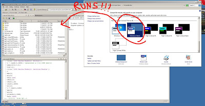
If you are having a problem where Matlab errors out on startup running Windows 7, try this it solved my issue.

Switch your "theme" to "Windows Classic" (right click desktop, select preferences, find the classic theme in the Basic and High Contrast Themes area)

Open Matlab. Enjoy.

Don't ask why... I didn't have time to research it. Seems to be related to Java.

Here are the some of the errors I was getting:
java.lang.NullPointerException
javax.swing.border.EmptyBorder.(Unknown Source)
com.sun.java.swing.plaf.windows.WindowsTableHeaderUI$XPDefaultRenderer.getTableCellRendererComponent(Unknown Source)


Wednesday, November 30, 2011

Adding a NE5532 Op Amp Model to LTSpice

To add the NE5532 Model, follow the steps in my LM741 post (see link below), using the NE5532 model shown here below.

Special thanks to Uwe Beis who provided the TI 5534 updated model:
(http://www.beis.de/Elektronik/Electronics.html)

Adding the LM741 model to LTSpice

***** NE5532 Source: Texas Instruments NE5534
* C2 added to simulate compensated frequency response (Uwe Beis)

* NE5532 OPERATIONAL AMPLIFIER "MACROMODEL" SUBCIRCUIT
* CREATED USING NE5534 model from Texas InstrumentsAT 12:41
* (REV N/A) SUPPLY VOLTAGE: +/-15V
* CONNECTIONS: NON-INVERTING INPUT
* | INVERTING INPUT
* | | POSITIVE POWER SUPPLY
* | | | NEGATIVE POWER SUPPLY
* | | | | OUTPUT
* | | | | |
.SUBCKT NE5532 1 2 3 4 5
*
C1 11 12 7.703E-12
C2 6 7 23.500E-12
DC 5 53 DX
DE 54 5 DX
DLP 90 91 DX
DLN 92 90 DX
DP 4 3 DX
EGND 99 0 POLY(2) (3,0) (4,0) 0 .5 .5
FB 7 99 POLY(5) VB VC VE VLP VLN 0 2.893E6 -3E6 3E6 3E6 -3E6
GA 6 0 11 12 1.382E-3
GCM 0 6 10 99 13.82E-9
IEE 10 4 DC 133.0E-6
HLIM 90 0 VLIM 1K
Q1 11 2 13 QX
Q2 12 1 14 QX
R2 6 9 100.0E3
RC1 3 11 723.3
RC2 3 12 723.3
RE1 13 10 329
RE2 14 10 329
REE 10 99 1.504E6
RO1 8 5 50
RO2 7 99 25
RP 3 4 7.757E3
VB 9 0 DC 0
VC 3 53 DC 2.700
VE 54 4 DC 2.700
VLIM 7 8 DC 0
VLP 91 0 DC 38
VLN 0 92 DC 38
.MODEL DX D(IS=800.0E-18)
.MODEL QX NPN(IS=800.0E-18 BF=132)
.ENDS

Monday, November 21, 2011

LM741 Datasheet


Many student projects use the LM741 op amp. Here is a link to the datasheet.


http://dl.dropbox.com/u/30278073/LM741_Datasheet.pdf

Wednesday, October 26, 2011

Thick Lines in LTSpice


Ever wonder how to thicken up the lines in your schematic or simulations? Turns out this is really easy.

1. Open the control panel (tools menu bar)
2. To thicken the schematic lines, Select the Drafting Options tab and check "Draft Thick Lines"
3. To thicken simulation lines, Select the Waveforms tab and check "Plot data with thick lines"

Wednesday, October 5, 2011

Exporting Data from LTSpice


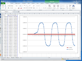
LTSpice waveform data can easily be exported for use in other graphing software like Excel.

To do this:

Step1: Run simulation, select File -> export
Step2: Select the traces of interest
Step3: A text file is saved in the LTC->LTSpiceIV root directory, the title will be "Draft1" by default or enter a desired file name.
Step4: Open the text file in Excel, or cut/paste from the text file

Wednesday, September 28, 2011

Parameter Sweeps in LTSpice - The .step Command

To step a parameter in LTSpice, simply place curly brackets around a variable name for the value you wish to step. We need to tell spice that we want to "step a parameter". To do this we us the "parm" syntax after the .step command. We need to tell the step command the parameter (variable) we want to step, the starting and ending value and the step increment.

Example: Let's say we want to step the value of a resistor from 10 to 100 ohms in 10 ohm steps. For the value of the resistor we use {R1}. Next, we use the ".step" spice directive followed by the step range and increment. We place the following directive on our schematic:

.step param R1 10 100 10


Here is an example stepping a voltage supply: