The Compute Spectrum Function

This function uses the FFT algorithm to compute the spectrum of an input with a number of points:

function [X,f]=ComputeSpectrum(x,fs,N);
% ComputeSpectrum Compute the Spectrum
%
% x input signal
% fs Sampling frequency of the input signal
% N number of points to evaluate spectrum (integer number of 2)
%
% X Absolute value of the spectrum (capital X for spectrum)
% f Frequency axis of the spectrum
%
% This function uses the FFT algorithm to compute the spectrum of an
% input signal with a number of points (N) N-point FFT where N must be
% a power of 2 (e.g. 2^10)
%
%Example: Compute the spectrum of sinusoid at 3Hz, fs=36Hz
%
% x=cos(2*pi*3*[0:12*3]*1/(12*3)); 12 times max freq
% [X,f]=ComputeSpectrum(x,12*3,2^12);
%
%Revision:0.0.1 jeastham
%
X=abs(fft(x,N));
f=(fs/N)*[0:N-1]; %make the axis freq
X=X(1:end/2);
f=f(1:end/2);

DSP Tutorial #4: Plotting Complex Signals

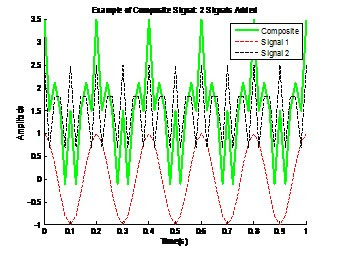
In this example we will plot a more complex time domain signal in Matlab:



clear all; %clear all variables
fs = 50; % sample freq
Ts=1/fs; % sample period
n=0:1*fs; % time window (fs=samples per second), 1 second
tn=n*Ts; % sample index
sig_a=cos(2*pi*5*tn);
sig_b=1.5+cos(2*pi*20*tn);
x=sig_a+sig_b;
% Time domain plot of x(t)=cos(2*pi*5*tn)
figure('Color',[1 1 1]);
h=plot(tn,x,'g','LineWidth',3);box off;hold on;
plot(tn,sig_a,'--r','LineWidth',2);
plot(tn,sig_b,'--k','LineWidth',2);
title('Example of Composite Signal: 2 Signals Added');
legend('Composite','Signal 1','Signal 2');
xlabel('Time(s)');
ylabel('Amplitude');
figure('Color',[1 1 1]);
plot(tn,sig_a);
title('Stem Plot Example: Fs = 50 (50 Points)');
axis('tight');

Sum of Sinusoids Triangle Approximation

Triangle Approximation: Sum of Sinusoids Example

The following Matlab code provides an example of the fact that any signal can constructed using a sum of sinusoids.



clear all; %clear all variables
fs = 50; % sample freq
Ts=1/fs; % sample period
n=0:1*fs; % time window (fs=samples per second), 1 second
tn=n*Ts; % sample index
wave_1=sin(2*pi*5*tn);
wave_2=sin(-1/9*sin(6*pi*5*tn));
wave_3=sin(1/25*sin(10*pi*5*tn));
wave_4=sin(-1/49*sin(14*pi*5*tn));
wave_5=sin(1/81*sin(18*pi*5*tn));
wave_6=sin(-1/121*sin(22*pi*5*tn));
wave_7=sin(1/169*sin(26*pi*5*tn));
x = (8/(pi^2))*(wave_1+wave_2+wave_3+wave_4+wave_5+wave_6+wave_7);
% Time domain plot of x(t)=cos(2*pi*5*tn)
figure('Color',[1 1 1]);
h=plot(tn,wave_1,'--r',tn,wave_2,'--k',tn,x,'g','LineWidth',2);box off;hold on;
xlabel('Time(s)');
ylabel('Amplitude');
title('Square Wave Approximation');
axis([0 1 -1.5 1.5]);

Plotting a Discrete Time-Domain Signal in Matlab

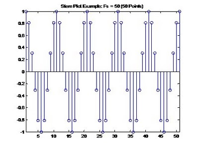
In order to properly construct a sinusoid in Matlab we need to do a few things. We need to give Matlab the equation of our sinusoid. We also need to tell Matlab how often to sample the sinusoid and for how long we want to sample our sinusoid. Essentially, we want to tell Matlab “ok, watch this 5Hz sinusoid for 1 second. In that one second, take 50 discrete samples (actually 51), and plot the data. I should see a point every 0.02 seconds, for a total of 51 total points (Matlab starts at zero).” What we want to do may seem pretty simple but this process often confuses students. This overview will help in understanding the proper construction of sinusoids. I say “proper” because we will use the proper DSP terms when we tell Matlab what to do. For example, we will use terms like “sample frequency” and “sample period” to describe our signal.

To establish our signal we will need to:

1. Set the sample frequency FS
2. Set the sample period Ts
3. Set the time window (number of samples)
4. Set the sample index Tn (time index)
5. Establish the signal x(t) and plot
   
   

1. Set the Sample Frequency (Fs):

This is our sample frequency. This is basically how many “points” we will use to construct each signal. Remember it’s zero based, so it’s really plus one. In the example below, Fs was set to 50, so we have 51 points in our plot, we ‘sample’ the signal 51 times. This is a 5Hz signal, so we are sampling it 10 times per cycle, which satisfies Nyquist-Shannon’s sampling theorem.

Matlab code:

Fs = 50;

2. Set the Sample Period (Ts):

Next, we will set the sample period, Ts. The sample period is calculated as 1/Fs, or 1/50 in this example = 0.02. This is essentially the ‘granularity’ of our sampling. In other words we will have a discrete point every 0.02 units (which will be time). If we zoom into our signal and only look at the first 0.2 seconds, we can see that we have 11 datapoints, one data point every 0.02s (remember it’s zero based).

Matlab code:
Ts = 1/Fs;

3. Set the Time Window (n):

Next we will establish out how many points are in one second of our signal. We will setup a matrix from zero to one second. In our example Fs = 50, so n = 0:1*Fs. When we set n in Matlab, all we are really doing is setting up a matrix of numbers from 0 to 50. That is: 0,1,2,3,4,5,6,…..,50. We will use this matrix to set the sample index Tn in the next step.

n is now equal to the matrix below:

0 1 2 3 4 5 6 7 8 9 10 11 12 13 14 15 16 17 18 19 20 21 22 23 24 25 26 27 28 29 30 31 32 33 34 35 36 37 38 39 40 41 42 43 44 45 46 47 48 49 50

Matlab code:
n =0:1*Fs;

4. Establish the Sample Index (Tn):

Now we will tell Matlab how to chop up or signal. We set the Sample Index as Tn = Ts * n. In our example, Tn will equal .02. We want to see a discrete point every 0.02 seconds. We will take n, or matrix from 0 to 500 and multiply it by Ts which was 0.02. Now we have a matrix with 51 elements from 0 to 1 spaced every 0.02 seconds. We are now ready to plot our sinusoid.

Tn is now equal to the matrix below:

0 0.0200 0.0400 0.0600 0.0800 0.1000 0.1200 0.1400 0.1600 0.1800 0.2000 0.2200 0.2400 0.2600 0.2800 0.3000 0.3200 0.3400 0.3600 0.3800 0.4000 0.4200 0.4400 0.4600 0.4800 0.5000 0.5200 0.5400 0.5600 0.5800 0.6000 0.6200 0.6400 0.6600 0.6800 0.7000 0.7200 0.7400 0.7600 0.7800 0.8000 0.8200 0.8400 0.8600 0.8800 0.9000 0.9200 0.9400 0.9600 0.9800 1.0000

Matlab code:

Tn =Ts*n;

5. Plot our 5Hz Sinusoid:

Plotting our sinusoid is pretty easy at this point. Remember, we want a 5Hz cosine signal constructed of 51 points in one second; we want to “watch” the signal for 1 second and plot the results. We can plot the X axis correctly with time also using tn.

clear all; %clear all variables

fs = 50; % sample freq

Ts=1/fs; % sample period

n=0:1*fs; % time window (fs=samples per second), 1 second

tn=n*Ts; % sample index

sig_a=cos(2*pi*5*tn);
figure('Color',[1 1 1]);

stem(tn,sig_a);

title('Stem Plot Example: Fs = 50 (50 Points)');

axis('tight');

DSP Tutorial Matlab Script

The script below will get you started plotting basic time domain signals. The following tutorials are available on additional DSP topics:

• DSP Tutorial #1: Basic Plots
• DSP Tutorial #2: Signal Creation
• DSP Tutorial #3: Sum of Sinusoids
• DSP Tutorial #4: Complex Signals
• DSP Tutorial #5: Frequency Analysis
• DSP Tutorial #6: Looping
• DSP Tutorial #7: Audio Processing
• DSP Tutorial #8: Spectrum Function
• DSP Tutorial #9: Basic digital filter
• DSP Tutorial #10: Windowing

This is a simple Matlab script which describes the basic plotting of time-domain signals.

%% DSP Tutorial Script
% James Eastham
% Member, IEEE
% Created on: 01/08/2010
% Revision: R1

%% Plotting a Basic Time Domain Signals
% Sinewave with a peak amplitude of 1 and a fequency of freq
clear all;
close all;
freq = 5; %5Hz
n=0:.01:.2; %number of discrete values on X axis
x = cos (2*pi*freq*n); %our cosine signal
figure('Color',[1 1 1]);
plot(n,x);
title('Example of Tim-Domain Signal');
xlabel('Time(s)');
ylabel('Amplitude');

%% Plotting a Basic Time Domain Signal Continued
figure('Color',[1 1 1]);
stem(n,x,'--rs','LineWidth',2,'MarkerEdgeColor','k','MarkerFaceColor','g','Markersize',10);
hold on;
plot(n,x);
title('Example of Time-Domain Signal Plot');
xlabel('Time(s)');
ylabel('Amplitude');


%% Plotting with the Subplot Feature
% subplot(m,n,p) breaks the figure window into an
% m-by-n matrix
figure('Color',[1 1 1]);
subplot(2,1,1);
plot(n,x);
title('Example of the Time-Domain Signal');
xlabel('Time(s)');
ylabel('Amplitude');
ns=1:length(n);
subplot(2,1,2);
stem(ns,x,'.r');
title('Example of the Descrete Points');
xlabel('Descrete Sample');
ylabel('Amplitude');
axis([1 21 -1.2 1.2]);
grid on;

Modeling Temperature in LTSpice - Part I

We can model temperature behavior in LTSpice using the built in step function.

To model a list of temps, insert the spice directive ".step temp list "
example: .step temp list -25 -10 10 20 25 50 75

To model a sweep, insert the spice directive ".step temp "
example: .step temp -55 125 25

The following example models a simple transistor amplifier from -55C to 125C in 25C steps.



The transient analysis below shows the source current over temperature.

Modeling Diode Reverse Breakdown Voltages in LTSpice

The included models in LTSpice do not include reverse breakdown. In order to model the reverse breakdown "vrev" can be specified in the diode model. For this example, create a new schematic and call the diode "mydiode". Insert the .model directive to add the reverse breakdown. Below, I used all the standard parameters for the 1N4148 and added vrev=50. The vrev specifies the reverse breakdown at -50V. Many other diode properties can be defined in the model including the non-linear characteristics of the breakdown.

Forward and reverse breakdown and current limitations can be modeled by using a more sophisticated model. Using the model below, forward and reverse current limiting can be observed.

.model mydiode D(vrev=40 Ibv=20nA BV=40 Ibv=1e-10 Is=1e-7 Rs=10 Tt=2n Ilimit=5mA Vpk=40 Revilimit=5mA)